Anybody working in PPC marketing should understand the power of Excel and the hundreds (or even thousands) of different uses it has that can make your life that little bit easier. As I’m sure you are aware, Excel is part of the Microsoft Office suite and is used primarily as a spreadsheet tool.
As the Office suite has developed over time Excel has also developed with it and is now much more than a simple spreadsheet tool with a built in calculator like it was in its first release. The functions that Excel now offers to its users almost abolish the need for the user to perform any manual calculations and as long as your formulas are correct and your raw data is correct, the output from Excel will be completely free of human error. As we know, when we extract a PPC campaign from Google, we are often presented with a csv file that is often over 100,000 rows with all the keywords and ad texts. If we had to manually go through these sheets without the assistance of Excel and change bids or certain URL’s then we would literally be there for days or even weeks.
Without a tool such as Excel it is unlikely that pay per click marketing would even exist as there would be no way to accurately and efficiently make calculated bulk changes to accounts based on specific criteria (something that any PPC marketer knows is vital).
So to celebrate all things Excel and thank our lucky stars that we have a program that enables us to put down the abacus I’d like to list my top 5 Excel functions & then go on to talk about how Excel can be used to automate the production of your Google Adwords ads.
1 – SUM
I thought we’d start with an easy one (don’t worry – they will get harder!) The Sum function does exactly what it says on the tin. It sums up whatever you tell it to.
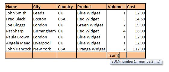
We always start our formula with =”function name” (in this case =Sum). From here we can select whatever data we want. We can do this in one of two ways. Firstly with “=sum(” in the text bar we can click in the first cell we want to sum up and then drag the mouse down through all the cells we want to sum up (this is called an array) or alternatively we can hold the ctrl key down and click in each individual cell we want to sum up – therefore selecting individual cells that aren’t necessarily grouped together in array.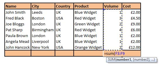 Above is an array style sum
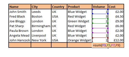
And this is an individual cell – notice how we are only summing up cells F3, F5, F7 & F9 whereas in the array style we are summing up all cells from F3 – F9. The result of the array would be 14 and the result of the individual cells would be 6.
2 – IF
The IF function in my experience is the most commonly used logical function in Excel. The purpose of the IF function is to specify a logical test to perform.
The structure of an IF formula in its simplest form is as follows =IF(Cell A=Cell B,”Value if True”,”Value if False”)
So let’s have a look at this in our example.
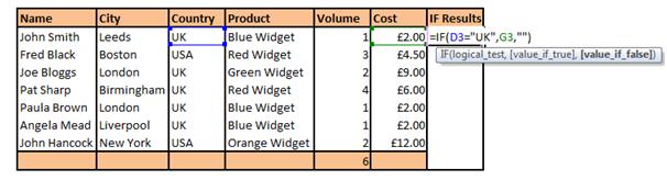
In the formula above you can see I have added on a column called IF Results and I have written a formula that will populate the new column with the cost of any products bought from customers in the UK. The formula in human terms states if the country = UK then bring back the value from the cost column otherwise bring back nothing. So if we drag that formula down the column our spreadsheet looks like this:
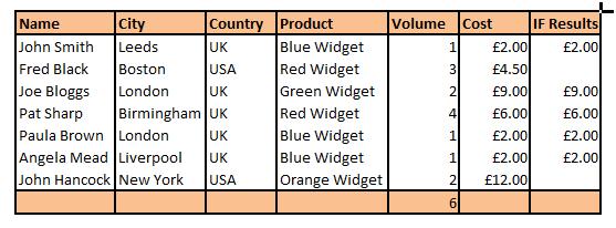
You can see that only the values of all the UK sales have been populated in the IF Results column. Obviously this is a very straightforward example of how to use the IF function. However when we combine it with other functions we are able to extract very complex data from our spreadsheet and populate cells based on strict criteria.
Other common uses of the IF Function are:
- IF Cell A is > (greater than) X,Value if True, Value if False
- IF Cell A is < (less than) X, Value if True, Value if False
- IF (AND(Cell A is > X,Cell A < Y, Value if True, Value if False (this logical statement says if cell A is greater than X but less than Y)
3 – VLOOKUP
This is without doubt the most commonly used lookup function used in Excel. Vlookup or Vertical Lookup to give it its full name is a powerful function that in the language of Microsoft looks in the first column of an array and moves across the row to return the value of a cell. In our terms it means that we tell Excel to look down the first column of a table and find the value we specify, then tell it to return the value on that row from a specified column. This function is usually used with large volumes of data where manually finding values would take hours. Let’s have a look at the structure of a VLOOKUP:
=VLOOKUP(Lookup Value,Table Array, Column Number, Match Type)
So let’s see an example:
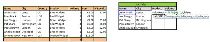
In the example above we have our original sales report with all the data from all countries. Now lets say that we were given a spreadsheet for UK sales that only contained the name and the City of those people that bought from us in the UK. We need to populate the product and volume columns with figures from our original sales report. Sure in a spreadsheet this size that would be easy to do manually, however when we have 10,000 sales in a month it is not so easy to do manually! This is where the VLOOKUP becomes a god send. In our example above our formula reads:
=VLOOKUP(J4,$B$3:$H$10,4,false)
This translates to:
Lookup Value = J4 (John Smith)
Table Array = $B$3:$H$10 – That is the whole of the original sales table (the $’s are used as place holders)
Column Index Number = 4 – this is the number of columns across the table array where the value you want to return is located. In our instance the product column is the 4th column along the table.
Match Type = False – This is normally set to False which means that the value the vlookup finds has to be an exact match of the lookup value.
So that would populate the product column – in order to populate the volume column we simply use the exact same formula again but change the column index number from 4 to 5 because volume is the 5th column in the table array. Our final output would look something like this:
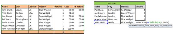
I have changed the order of the names in this example to show that it doesn’t matter what order your lookup values are in.
So now we have our bases covered with the 3 most commonly used functions let’s step it up a gear and look at the SUMIF and SUMIFS functions.
4 – SUMIF & SUMIFs
SUMIF – A great function in excel that allows us to sum up values based on logical expressions or as Microsoft put it Adds the cells specified by a given criteria.
SUMIFS – Much the same as sum if but this function allows us to sum cells based on multiple criteria.
I’m sure that any PPC marketers out there know how much of our time is spent reporting on our clients sales figures. Often these sales figures are handed over from the client in one long spreadsheet that lists all the sales since the company began trading. This is great to have all the information in one place but it can be a bit of pain for the analyst who needs to see quickly and easily how many sales were achieved in a certain month for a certain brand for instance. This is particularly common when creating weekly or monthly reports for our clients that show how our PPC campaigns have affected their sales.
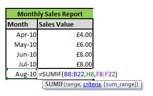
The structure of a sumif statement is as follows:
=SUMIF(range, criteria, sum range)
Range = this is the range from your raw data where you want the criteria that you specified to match for example if you are looking for a certain month your range would be the month column of your raw data.
Criteria = This is the value you want to find. It could be anything really from a month to a number to a word.
Sum Range = This is the range of numbers you want to sum up based on the criteria you specify and will be in your raw data sheet.
Let’s look at a quick example of Sumif in action:
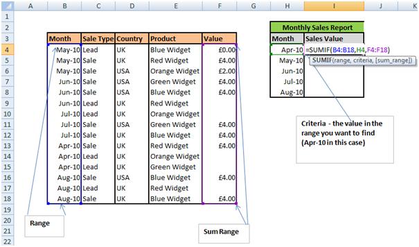
The formula in cell I4 is looking down column B in the raw data and summing up anything in column F where Column B matches H4. In other words the formula looks down column B for the date Apr-10 and sums up the value in column F when it finds it. The Result of this will be £4.00 because in April there is only one sale and it is worth £4.00. To fill the rest of this column we simply have to drag down the formula to the bottom of the table. And the results will look like this:
Now we know how a SUMIF works let’s look at SUMIFS. SUMIFS work very much the same as the SUMIF function but they allow for multiple criteria. The basic layout of a SUMIFS function is as follows:
=SUMIFS(sum range, criteria range 1, criteria 1, criteria range2, criteria 2 …..)
Let’s look at this in action:
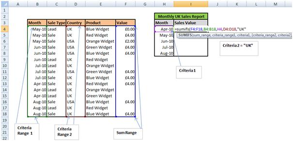
In the example above we want to sum up the sales value of all UK Sales by Month. As we can see in column D we have both the UK and the USA so this needs to be specified as a criteria in our formula and is done by specifying the criteria range 2 as the country column in our raw data (D4:D18) and then actually typing in what we want it to find in quotation marks –”UK”. Our final output looks like this:
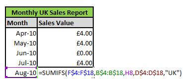
As you can see from the output our results only show the sales value for the specified month based if the sale comes from the UK.
5 – FIND Function
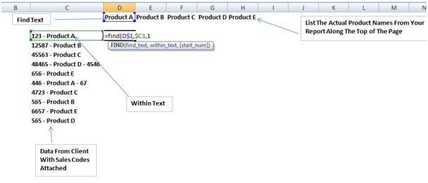
The Find function is a particularly handy tool for PPC marketers to have in their arsenal. This function allows the user to search inside a text string in another cell and if it finds the value it returns the starting position of the value within that cell.
The structure looks like this:
=FIND(find text, within text, start num)
In simpler terms this means = FIND(Value you want to Find, cell you want to look in, position in the text string you want to start the search from – usually 1)
This is a great replacement for VLOOKUP when the values you are searching don’t match exactly. I find this is used a lot when we receive data from clients and certain aspects of the report don’t match – for example – their product names may have a sales number attached to them. This makes the VLOOKUP function redundant because it will only find instances where the cell matches exactly.
Let’s look at this example where we have received some raw data from our client but the product names have a number attached to them. We know the products as Product A, Product B, Product C etc and our report needs the data to be named in that manner to execute properly.
When we fill this formula across the rest of our table we are left with an output that looks like this:
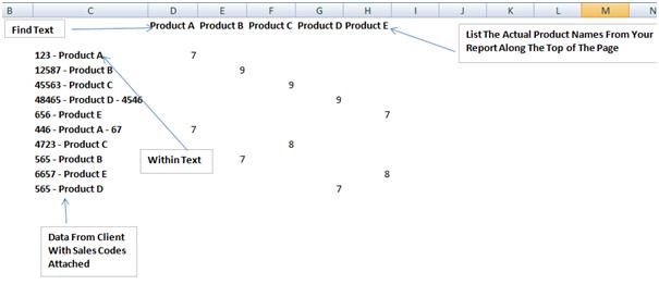
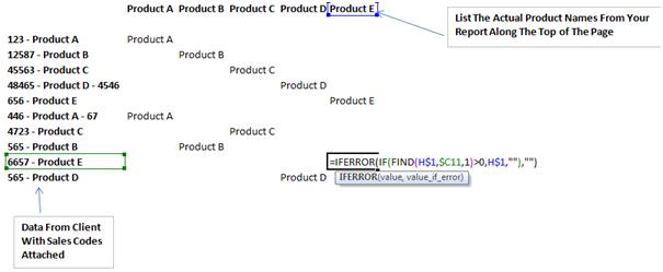
You are probably wondering why the spreadsheet is populated with what appear to be random numbers. Well the FIND function returns the starting position of the value you are looking for. So in Cell D3 above we see we have 7 – that is because the word “Product A” begins 7 characters in, in cell C3. So now we know which products are represented by the data but it is not ideal for us in this format. In this instance I would expand on our Find function by using an IF function.
It is worth mentioning that I added an IFERROR function to the formula so that we didn’t receive any error values in the table. The cells that would result in an error remain blank now.
Currently we have the formula =IFERROR(FIND(D$1,$C3,1),””).
If we change this slightly to =IFERROR(IF(FIND(D$1,$C3,1)>0,D$1,””),””) then our output is much more manageable. We have added an IF statement here that says if the result of executing our formula above results in a number greater than 0 then use the actual product name in cell D1 (Product A) & If it doesn’t result in a number greater than 0 then leave the cell blank. The output now looks like this:
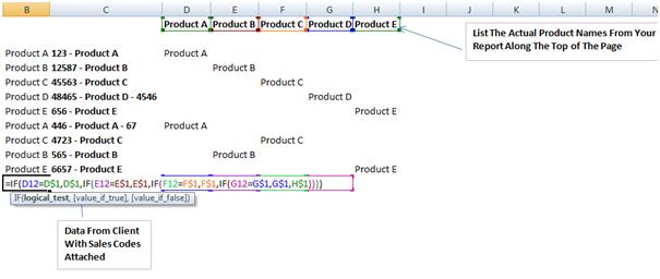
What you choose to do with the Data at this point is up to you but you are left with a table that clearly shows which product belongs to which sales record. Most likely you would replace column C with the correct product name so you can run your report correctly. This can be done by simply using this formula in cell B:
=IF(D3=D$1,D$1,IF(E3=E$1,E$1,IF(F3=F$1,F$1,IF(G3=G$1,G$1,H$1))))
This is called a nested IF statement & the formula basically checks across the row to see if the value in the cell matches the value we are using in our report and if it doesn’t then it moves onto the next column.
Our output looks like this:
So those were my top 5 functions that I use when analysing PPC campaign data. Of course there are many more useful functions in Excel that I use on a daily basis but I hope that these give you a good overview of what can be done with Excel. Why not practice combining functions within other functions and see how much easier your data analysis becomes.
The final part of this post is going to be a quick overview of how Excel makes it possible to automatically generate optimised ad texts for your Adwords PPC Campaigns. It is worth noting that this technique is not suitable for all PPC campaigns but can save a tremendous amount of time when used in the right circumstances. Usually e-commerce sites will be suitable for this technique:
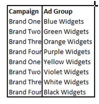
With larger e-commerce PPC campaigns we are often given a product feed from the client that lists every product they sell. These will differ quite drastically from one client to another but they will often contain rows similar to the one shown below. For this post we will assume that the PPC campaign structure is Brand Name for Campaign & Product Name for Ad Group.
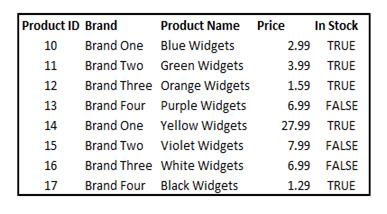
This is the beginning of our Ad Master Sheet:
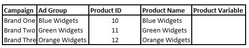
Our first step is to ensure that all our product names are less than 26 characters long. This is done using a simple =len formula. In our example none of our products are above the 25 character limit so we can leave that column unpopulated.
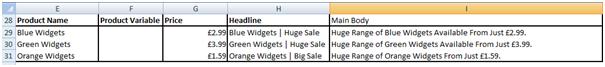
Our next step is to create a headline. We need to think about what we would most like our headline to say based on the length of the text string. To do this we need to create a lookup table like the one below:
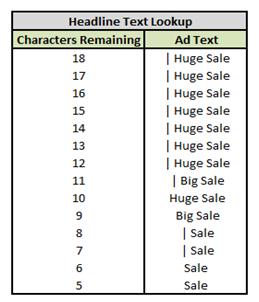
The table above shows the text string we would like to use in our headline based on the number of characters we have left after inserting the product name.
So our master sheet will now look a little something like this:
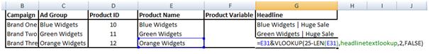
As you can see the headline text field has now been populated with the correct extension based on the number of characters that remained out of the 25 available to us.
Next we need to look at the main body of our ad text and what we want it to say. Again this should be based on the characters available to us. To do this you should start by creating a list in order of characters & preference.
E.g.
Huge Range of Product Name Available From Just Price.
Huge Range of Product Name From Just Price.
Product Name in Stock Now From Price.
You should create this list with a greater number of possible ad texts – I have only used 3 for the sake of this post.
I am going to say that I need the above to be below 55 characters long because I the longest call to action I would like to use “Buy Online Now” requires 16 spare characters. I may not be able to use that call to action in this example but I will explain that later.
There are several different formulas we could use here but I will use a nested IF statement and it will read something like this based on our running example:
=IF(LEN(“Huge Range of “&E29&” Available From Just “&G29&”.”)<55,”Huge Range of “&E29&” Available From Just “&G29&”.”,IF(LEN(“Huge Range of “&E29&” From Just “&G29&”.”)<55,”Huge Range of “&E29&” From Just “&G29&”.”,E29&” In Stock Now From Only “&G29&”.”))
The formula above basically looks at how long the output will be for each of the 3 different ad texts and selects the largest one that fits within the 54 character limit that I have available to me. As we can see the main body column has been populated with the suitable ad text so now we can use a little bit of VB script to separate the text string into a Google friendly size. I will not talk about VB script here but it is relatively straight forward to create a piece of code that will allow you to separate a text string into 35 character strings without dissecting words.
You should now have something that looks like this:
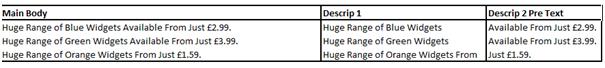
As you can see we now have our description line 1 and part of line 2. So in order to complete our ad we need to determine how many characters we have left in description 2 and choose the correct call of action from a lookup table. Here’s one I made earlier!
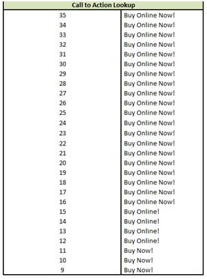
The formula we need in the next column reads something like this:
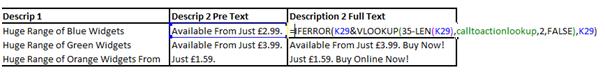
=IFERROR(K29&VLOOKUP(35-LEN(K29),calltoactionlookup,2,FALSE),K29)
In other words take description 2 pre text and add whatever statement in the lookup table relates to 35 – the length of description 2 pre text – in the first example below we were left with 9 remaining characters which meant that in the lookup table we were given the call to action “Buy Now!”.
There we have it – we now have a headline, description 1 & description 2 that can be easily changed and added to Google in a fraction of the time it would normally take to write out manually. It may seem like a lot of work to do just to write these ads but the time you will save in the long term far outweighs the time it will take to initially set this up. However you should bear in mind that this is only a brief example of how to set up Excel to write ad texts. In reality you should have much more variation in your headlines and ad texts and much more validation in place to ensure that your ads never go over the character limit and revert to the most basic text option.
I hope this has given you some insight into Excels features and functions and has shown you how useful it can be in your PPC marketing campaigns.