Building on my last blog post, I want to share a couple of intermediate tips that will help you deliver some more complex and bodacious reports for your PPC Data in Excel. The last post covered how to set up a structure to a PPC account that would work with Excel and showed you a few techniques to implement and manipulate this in order to create custom reports. If what you had before was a plain all-mountain board, here are a couple more tips to allow you to tweak the set-up, and get you comfortable and ready to test some advanced tricks.
Using Named Functions To Cruise Through Deep Data
As with the structure of your AdGroups, apply a good naming convention to your Excel functions. Keep things simple and short but readable. A good method to follow is to prefix a value to identify the types of references. This will certainly help as you expand the scope of your report and develop your own knowledge of Excel. For example, I would prefix the terms “query”, “value”, “selector” or “series” where appropriate.
From there on creating names that work in simple patterns will help expedite your own development time, especially when building charts and advanced calculations. The bottom line is not to complicate things: “seriesImpressions” will work just fine. Then as you build sets of similar calculations, you will be able to read and track your work easily, and simple find and replaces will get our processes up to speed.
If nothing else this will be your way to blaze through fresh tracks, leaving killer tracks for the grommets and guiding your next lines as you start to branch out.
Introducing Excel Forms & User Control
Excel forms are in part some of the easiest introduction to VBA development you will ever get, and a great way to free the reins on your data. Checkboxes will return a Boolean value of either TRUE or FALSE and these can be used as 1 and 0, respectively, in calculations. When inserting a checkbox, right click, format the control and use the cell link. This will then return the value of the checkbox in that cell allowing you to create a formula name for the cell. A handy tip is that the value of the checkbox can now be changed by inputting the values “TRUE”, “FALSE”, 1 and 0 into the linked cell.
Another great way to use forms is by combing radio buttons with the CHOOSE function. Radio buttons work in groups, and all buttons in one group should be linked to the same cell. Once they are inserted into your spreadsheet, select them all, right-click, format and link the cell. At this point you can test your buttons and you will see that only one button can be selected at a time, producing a unique number in the linked cell.
As these number values are incremental by 1, they can be used to call a unique value from the CHOOSE function. This function allows Excel to pick a unique value by an index number. If we say the linked cell “selector” is producing our index number either 1 or 2. We could create a function
= CHOOSE ( selector , “A” , “B” )
So that when “selector” = 1, the function will return A.
Using this within PPC we are able to create series and data sets with variables linked to our CHOOSE function. One example would be to have our “selector” CHOOSE between Click-Through-Rate and Conversion Rate like so:
= SUM ( CHOOSE ( selector , dataClicks , dataConversions)) / SUM ( CHOOSE ( selector , dataImpressions , dataClicks))
Here, if “selector” = 2, the function will return the SUM of Conversions divided by the SUM of Clicks giving our Conversion Rate.
Tweak and Style Charts with User Controls
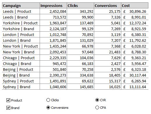
When you deploy Charts with your User Controls you can start to cram a heck of a lot of data into a single chart. Take the following PPC Report, and using techniques covered earlier in this post and my previous blog we are able to create series of data and tests to implement the controls beneath.

Our naming convention allows us to create a test series quite easily. To the cells to the right of the data break down the Campaigns by location: Leeds, Yorkshire etc. In each cell of the series you want to input the following formula:
= IF (ISNUMBER ( SEARCH ( “Product” , dataCampaign )), IF ( selectProduct = TRUE ), CHOOSE ( selectorMetric ,dataClicks , dataConversions ), 0 ) , IF ( selectBrand = TRUE ), CHOOSE ( selectorMetric ,dataClicks , dataConversions ))
Using this framework we can then construct the rest of the data we will use to create the series for the chart.
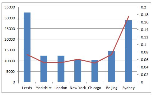
If we then create a list of the locations we can simply SUM our series data where dataLocation is equal to the name given in the list. This then creates a dataset which will create a simple but interactive column chart like this one:

Summary…
Moving on from the last post, we have now left the realms of how well Excel works with PPC data but into a point where Excel begins to prove itself as one of the best and most practical ways to deliver reports to clients. Such simple manipulation as covered in this post will allow you to create reports that can compile useful data from many campaigns, many accounts, and even many search networks and platforms into a simple and easy to use format. Having built that all-mountain board, we are essentially stepping off the piste and into park.


