Data is at the centre of all the decisions we make for our clients. One of the ways we do this is to use a statistical data analysis technique called time series decomposition, which allows us to undertake detailed analysis of search traffic and make better-informed campaign decisions.
In a previous blog we used time series decomposition in Excel to break down signals, such as traffic, revenue, search volume etc. into its component parts. Typically, we look to identify a ‘seasonal’ component (i.e. time-based cyclical trends), which may have predictable peaks and troughs over a set period, and the underlying growth rate over the long term.
In this blog, we set out some real examples of where time series decomposition has made a significant difference to the performance of our clients’ digital marketing campaigns.
Instead of using Excel, in these examples we use R, a piece of statistical software that is quick and simple to use.
Seasonal trends in PPC
Our PPC experts work to maximise returns on click spend over the year by considering seasonal search volumes and conversion rates and allocating budget appropriately. We use time series decomposition to guide our clients with budget planning for the next financial year, or when required to forecast performance over a given period.
In R, the “stl” function splits a signal into it’s seasonal, trend and noise elements, allowing us to view each separately. We load the data and convert it to a time series object using the following code:
myTimeSeries <- ts(myData)
splitSeries <- stl(myTimeSeries, s.window =”period”)
plot(splitSeries)
Using a sample data set, we can display the different elements as follows:
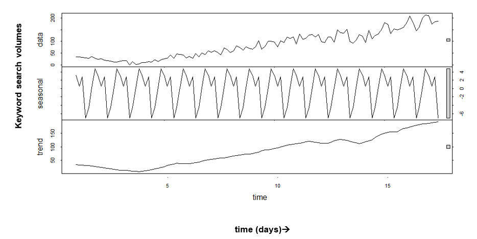
In this sample, we can see recurring trends in the ‘seasonal’ data, which we then analyse and use to adjust PPC budgets up or down to ensure we have the budget available to capitalise on peaks in search volume.
After ‘decomposing’ the data into its constituent parts, in this sample, we see the underlying traffic trend, with the seasonal fluctuations removed. This example shows an underlying trend of traffic growth, which might not always be the case.
Of course, we also want to make sure we catch traffic that is a result of growth, but we also need to work out:
- How much is this traffic worth to us?
- How much should we pay for these clicks?
Further segmentation would be necessary but, splitting out seasonal trends from growth traffic is a strong starting point.
Analysing growth in SEO campaigns
Another use for time series analysis is in assessing growth in isolation. Our clients want to know what the real picture is on their SEO activities: are they experiencing growth in traffic, or are seasonal fluctuations masking the truth?
Using the technique above, we can strip away the noise in the signal, and see the real patterns. This could also be done by calculating a moving average. The forecast package in R makes this very straightforward to do, and allows us to make an informed prediction:
arimaModel<- auto.arima(myTimeSeries)
library(forecast)
forecast(arimaModel,10)
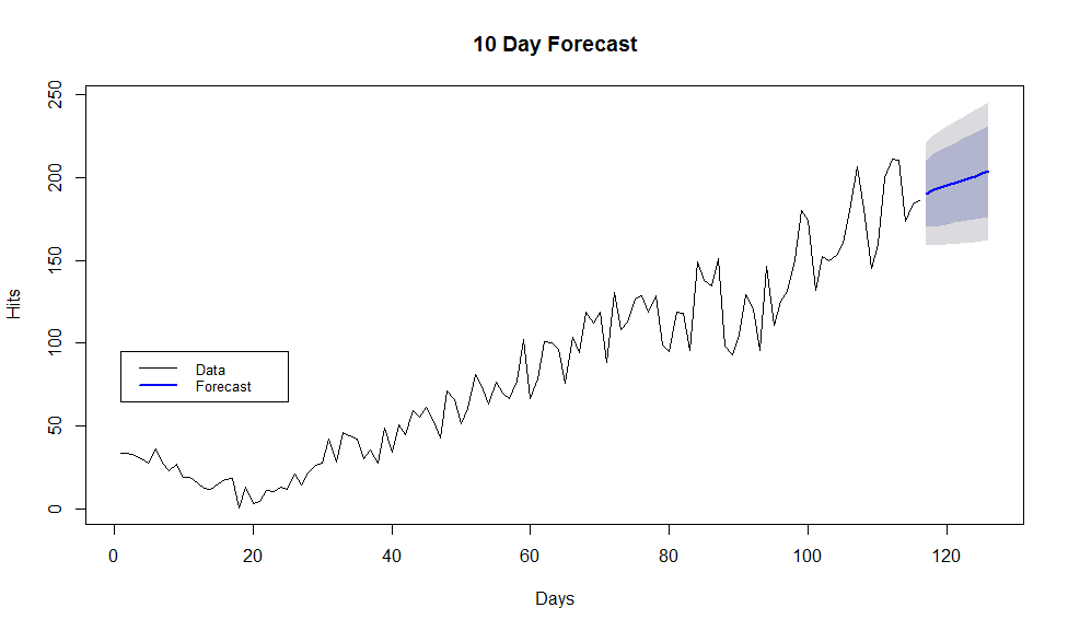
This plot shows our signal, and a projection for the next ten data points. If you are using daily data, it will show the next ten days, and if you are using weekly data it will plot the next ten weeks etc. This helps us look beyond seasonality and shows us whether our client is experiencing growth.
SEO forecasts
This method has also been useful in producing forecasts where a significant incident has affected a domain, and we want to know what would have happened without the effect of the penalty.
For example, if a site receives a manual penalty from Google – how much does that cost the business?
We can answer this by using time series analysis to forecast traffic and revenue from a point in time prior to the penalty being applied, up to the present day. We can then measure the difference between the forecast values, and the actual traffic or revenue, and get an idea of the severity of the penalty.
This can be useful where a lengthy process of link disavowal is required, as it shows the potential success of the website without the penalty and therefore the value of completing the link disavowal.
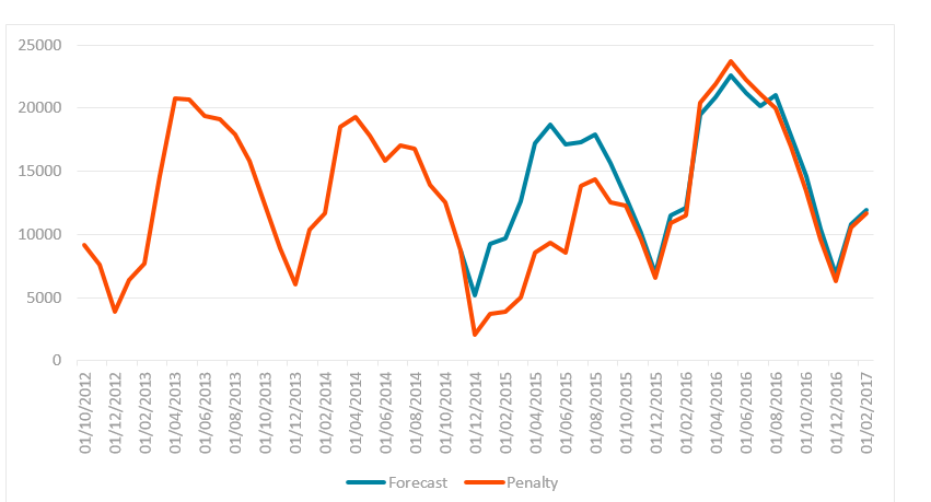
This chart shows traffic to a domain that received a manual penalty in December 2014. The orange line indicates the actual clicks to the site, the blue line is our forecast of what would have happened if the penalty had been avoided. This allows us to calculate the amount of lost traffic, and put a value on the work being done to have the penalty removed.
Summary
This type of statistical analysis can make a significant difference to digital campaign optimisation.
Using data science we can make evidence-based judgements, and time series decomposition is just one piece of statistical analysis that we use to get the best results.
Is your data being used effectively? Please contact us to find out more.
Further resources
For more info on using R for time series analysis, check the sites below:
https://a-little-book-of-r-for-time-series.readthedocs.io/en/latest/
https://www.r-bloggers.com/2014/04/time-series-analysis-using-r-forecast-package/
https://www.statmethods.net/advstats/timeseries.html