The problem
This is a specific piece of advice to solve a specific problem – slightly different to our other blogs. If you’ve found this blog there’s a good chance that, like me this morning, you are searching the internet for advice on using conditional formatting colours on a font rather than a cell background. It seems that the usual places hadn’t managed to crack this as various posts on excel forums asked the question and so far no one had answered it. Well, here is how to do it!
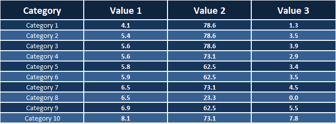
Perhaps you have a table like the above. Its hard to make the different values stand out against each other, or give an immediate impression as to how they range from low to high. Of course you could do this with a chart of some sort, but there are times you want to keep the table format. Conditionally formatting the number values based on their size is the obvious answer, perhaps making low values red, running through orange and yellow for medium, and green for high. Sadly its not obvious enough for Microsoft to have included it as an option!
The workaround
What you can do is fill in the cell backgrounds using conditional formatting, and that’s the first step in the workaround.
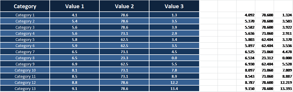
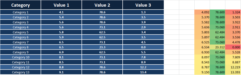
Set up another data range, copying the values from your table, elsewhere on the worksheet. Then simply apply the desired conditional formatting to this range. If you need help with this stage, thankfully there are other sites explaining this – see here for a good introduction.
What we need to do now is grab the colour index of each cell background, and we can apply those to the font. Using VBA (Visual Basic for Applications) exposes the hidden properties of many Excel objects, so my first thought was that we could write code to do this for us. Unfortunately, it appears Conditional Formatting behaves according to its own unique set of rules, and what we see above aren’t actual background colours, rather this data is handled differently – which means we cant get the colour index property! I spent a while trawling various sites this morning to find the answer to this before realising how easy it was.
The trick
Select and copy your range:
Open Word (can you guess where this is going)
Paste then immediately copy what you have just pasted. Pasting into Word destroys some of the formatting – the conditional rule is lost, and any formulae would be as well. However, the background colour – the result of the conditional formatting – is preserved, and is now stored as a background colour.
Paste your table back into Excel. You will be able to change a value now without changing the colour, as they are no longer conditional, but just colours. So we can write some code to use these colours and apply them to the font in our table. Before doing that, we need to name some ranges. Select the values in your table – just the cells with numeric data in them. Click into the address bar at the top left of your main Excel window, and type a name e.g. destRange. Then select the table we have pasted in from Word, and name it sourceRange. This will let us reference these ranges easily in code.
VBA code
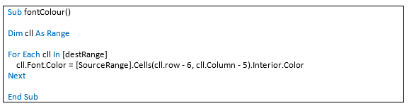
There are plenty of guides to using VBA around, and some other blogs on this site cover introducing it. I will assume you have at least some knowledge of using it. To open the VBE (Visual Basic Editor), press Alt + F11. In the project window, right click on your files name and choose Insert Module. In the module, paste the following code (note American spelling of Colour):
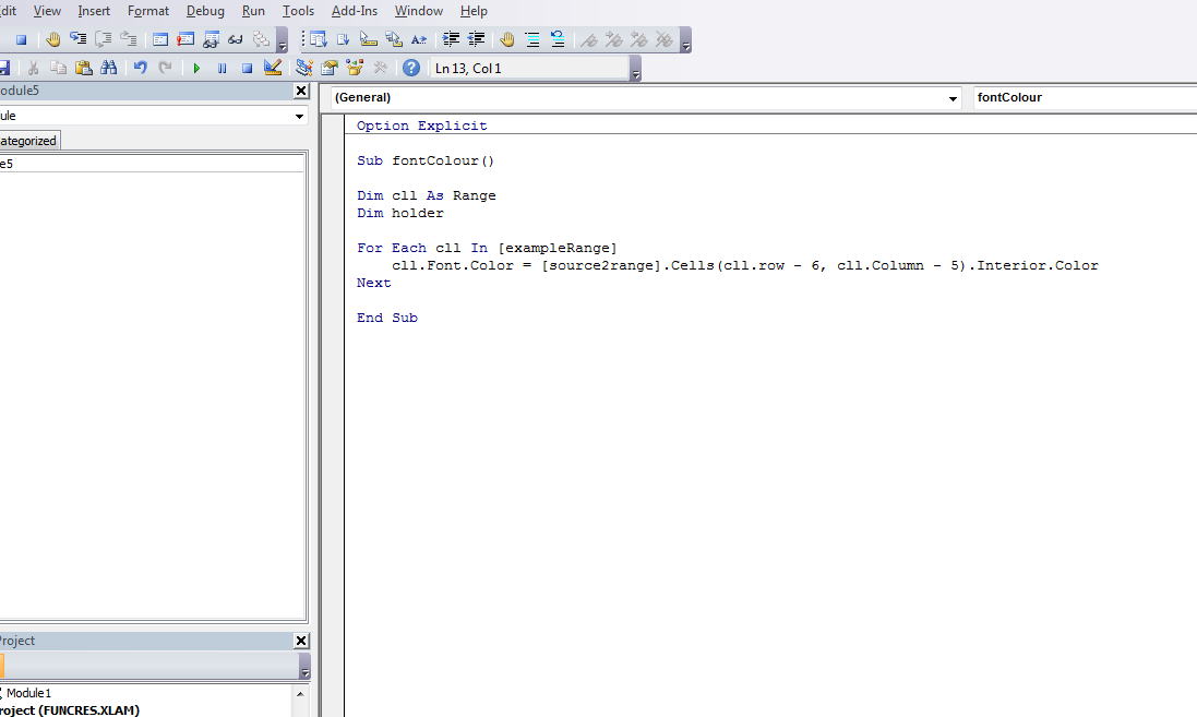
Your VBE should then look something like this:
What this code does is loop through each cell within the destRange – our data table. For each cell, it looks at the corresponding cell in the sourceRange, and changes the Font Colour property in the destRange to match the Interior Colour property of the source Range cell. You may need to edit the values in the Cells section.
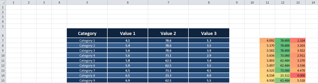
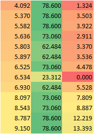
As you can see above, the value in 4.1 is in row 7, column 6 of the spreadsheet. The corresponding cell with the colour I want is in row 7, column 11. However, the line of code [SourceRange].Cells (row – 6, Column – 5) Interior.Color tells Excel to count the rows and columns within the range, so the top left cell is row 1, column 1. So, I must subtract 6 from the row value, and 5 from the column value to get the colour index from the top left cell. As the code loops through all the cells, the row and column numbers will increment and so the subtraction leads us to the appropriate cell each time.
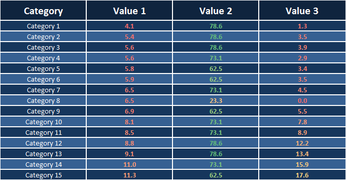
Once you are happy with the above, click within the code in the VBE and press F5. This will run the code. All being well, you now have conditionally formatted font colours, as below!
 For further help with VBA, check out these sites:
https://www.excel-vba.com/excel-vba-contents.htm
https://www.techonthenet.com/excel/formulas/index_vba_alpha.php